Python pandas tips to make your life easier

Introduction

Modern packages in Python might still surprise us in how many secrets and shortcuts they keep to make the developer’s work easy and optimized. Pandas, one of Python’s most recognized and widely used packages in recent years, is not an exception to this fact. Its capabilities in data analytics, finance, data modeling and artificial intelligence development cannot be underestimated. For a big part of the developers community, though, pandas keeps a plethora of hidden gems that may still remain unknown. In this article I would like to introduce a few examples of more or less advanced yet very simple tips of that package that will make a developer’s life much easier.

Categorize columns with data types

Memory optimization plays a vital role in software development. Same rule applies to working with the pandas package. It is surprising that not everyone is familiar with the fact that pandas offers a comprehensive collection of types to represent data in the DataFrame columns. In particular, a category type becomes essential as it enables significant memory optimization.

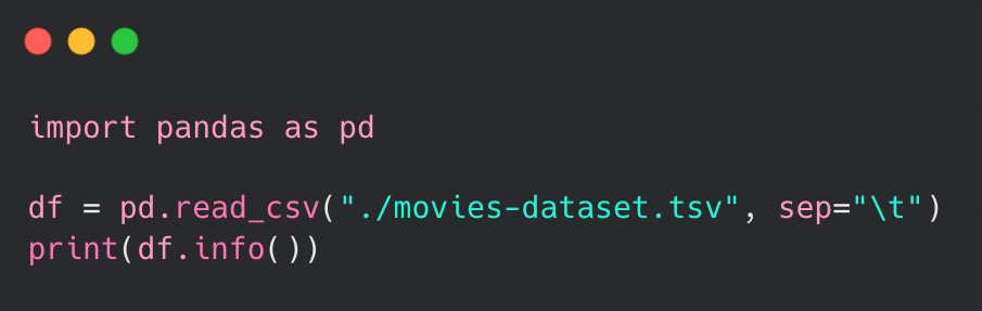
To show its capabilities, I have utilized a dataset that includes actors’ data of over 12 million rows. Subsequently, I loaded it into the DataFrame in order to display the results:

Below are displayed the results of the code execution. It provides insights into how pandas interpreted the input data and corresponding types employed to represent the created columns.

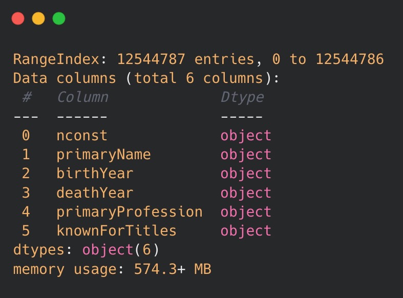
As one may see, pandas interpreted all the columns as objects, meaning that no particular data type has been assigned and resulting in memory usage of over 570 MB. This amount of memory consumption is undoubtedly high, thus optimization should definitely be applied.

This is where the utilization of data types in pandas becomes an essential advantage. By specifying a column type mapping within the read_csv() method, we can indicate expected column types of the DataFrame. In order to optimize the memory usage of a DataFrame, we might implement a categorical type, which is designed to represent a chosen column with a fixed number of unique values or categories. 

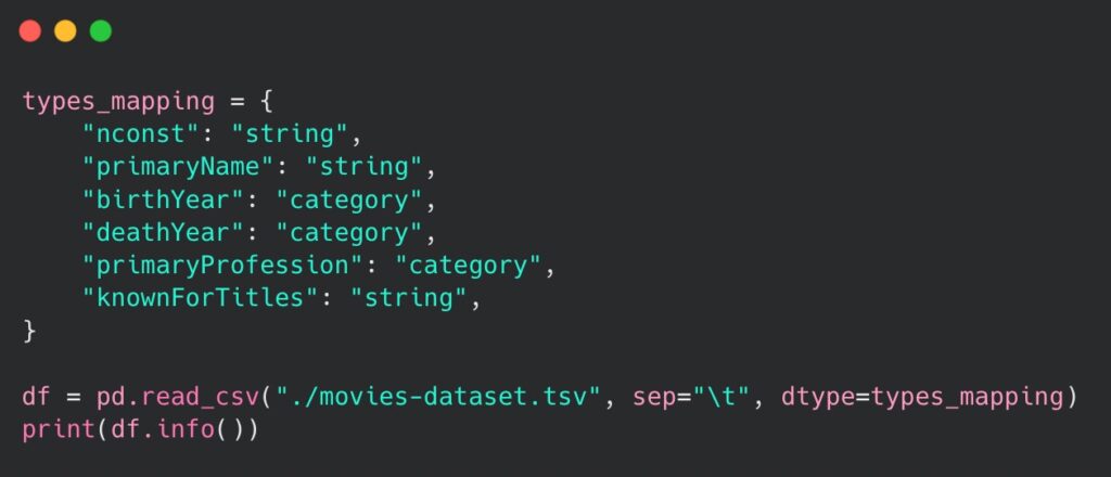
Declaring a category type is particularly beneficial when working with big datasets, where certain columns represent a limited set of values (e.g. gender, status, birth year etc.). In our example, we may try to use it on the following columns: birthYear, deathYear and primaryProfession. Therefore, we should be able to optimize the memory used in the loading process. The code to achieve this is as follows:

Type mapping could also be achieved by using a dedicated astype() method on the previously loaded DataFrame. Regardless of the approach, the result is as follows:

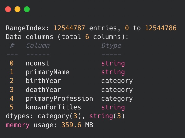
It is evident that implementing a categorical type has resulted in more than 200 MB of memory savings. The outcome of the code emphasizes the importance of utilizing category types, especially when working with large datasets that have columns containing restricted sets of values. 

Nevertheless, there are a few drawbacks to using them that all developers need to have in mind, in particular:

• Performance impact during conversion, since converting a column to the category type involves additional computation to create the categorical codes and build the mapping. 
• Limited operations and compatibility, as some pandas operations and methods might not be fully compatible with category type columns. 
• Immutability, since once a column is assigned the category type, the categories themselves are immutable. 

If the dataset’s categorical data is subject to frequent changes in their values, using the categorical type may not be the most suitable choice.

Use DataFrame.apply()

DataFrames come with a dedicated apply() method that accepts any function object (including lambda expressions) as a parameter to be applied into their columns.

Let us take a look at following code, that performs a salary raise to each employee within the DataFrame:

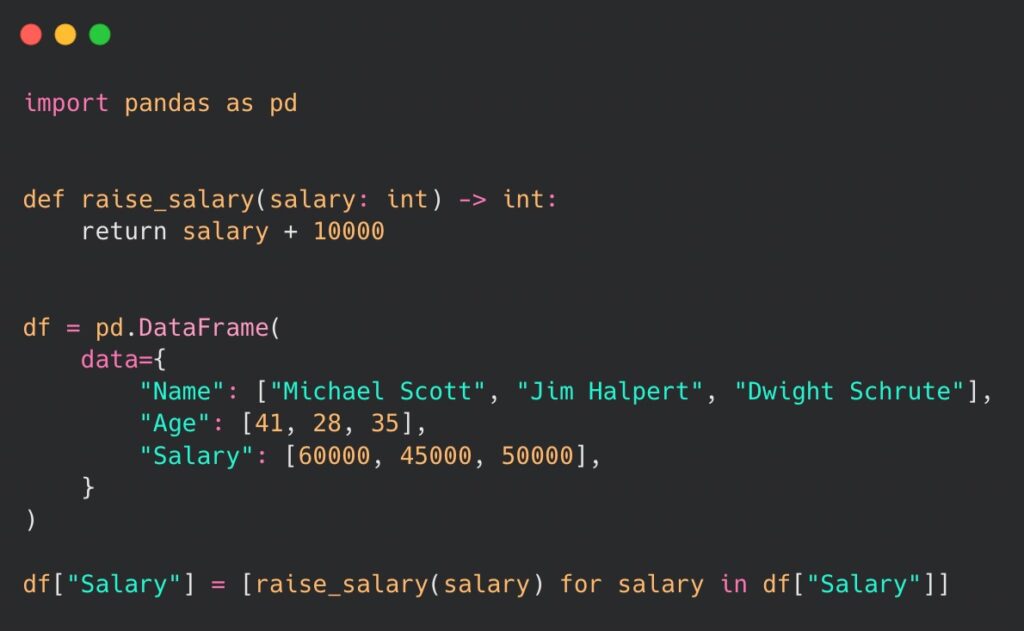
Above, we have used a list comprehension to apply the raise_salary() function to each value in the Salary column. The apply() method of the DataFrame allows to use custom functions on one or multiple columns and enables to perform element-wise operations or transformations on the included data. All it takes is a simple one line of code based on the  the example above:

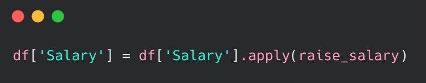
Not only does the code look more clean and well organized but we may also see an optimization in execution times for bigger sets of data. In our case, applying the same function to the DataFrame of 100k rows optimized the request by ~21%:

Using list comprehension	Using apply()
35.12ms	27.76ms

For bigger DataFrames or more complex transformation functions the results might further grow in favor of using the apply() method, thus making it a more optimized and elegant way of dealing with data manipulation.

Query your DataFrame

One feature that often goes unnoticed by many developers is a powerful query() method offered by pandas. It allows the filtering of data in the DataFrame in a very intuitive and readable way, mainly because of a simple, SQL-like syntax. It is a valuable tool for extracting subsets of data by providing a specific filter or criteria. Let us take a look at an example below:

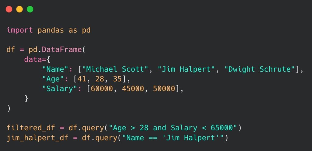
As one can see, by utilizing the query() method we have managed to retrieve rows where Age is above 28 and the Salary is below 65 000. Additionally, we have retrieved an employee of a specific name provided in the query formula. The code syntax for both operations is straightforward and readable. The query() method enables us to perform both simple and more complex queries, handling logical and comparison operators. The execution of the code is also very efficient and can enhance the overall performance of the application. Therefore, using the query() method should become a preferable way for data filtering in DataFrames.

Discover pivot tables

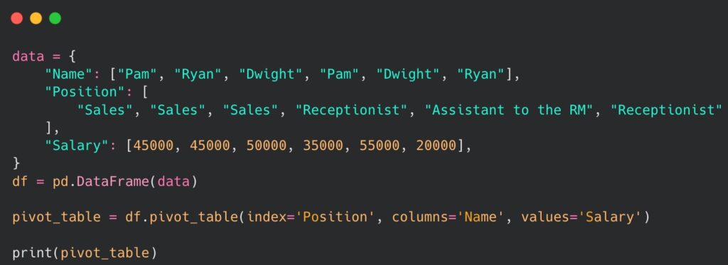
When grouping and summarizing the data is our main goal, pivot tables may become an essential tool to perform the work. Their main purpose is to represent the given DataFrame in an aggregated and reshaped way by creating a new table with a data summary. Pivot tables consist of an index column, a set of columns to be used for table creation, values to summarize and (optionally) an aggregation function to be applied to the data.  A code snippet below will show the results of using the pivot table.

The result of the code execution is as follows:

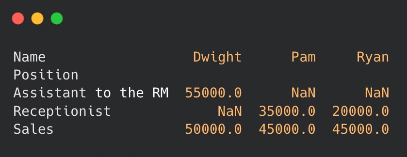
As one can see, pandas pivot table effectively presents a summary of employee salaries, while also highlighting the salary changes for particular individuals as they progressed in their positions. A possibility of implementing aggregation functions such as sum, count or median is a worth mentioning addition, perfect for in-depth data analysis. Clear and simple data representation makes pivot tables a versatile tool and an ideal solution for presenting and summarizing statistics based on the specific needs of the analysis.

Create custom and multi indexes

Another noteworthy feature is the customized index implemented in pandas. Custom indexes enable more meaningful labels, non-numeric indexing, and enhanced indexing operations. By utilizing them we may improve the readability of our data, allow non-numeric index values (such as tuples or datetimes) and apply more intuitive retrieving of DataFrame subsets.

Let us take a look at an example of using a customized index:

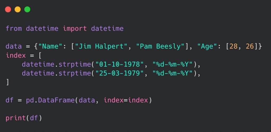
In the example above, we were able to apply a datetime-type “day of birth” as a custom index to the existing employee data instead of regular numeric values. The results of that operation is following:

When a more hierarchical structure or more advanced selection and grouping operations are required, one might consider using a MultiIndex feature of the DataFrame. It allows the creation of DataFrame and Series objects with multiple levels of row and column labels in order to organize data that has multiple dimensions or a hierarchical structure. Each level of the index labels may represent a separate dimension or grouping of the data. Let us take a look at an example below:

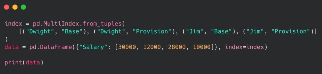
The implemented MultiIndex allowed differentiation between the “base” salary and “provision” received by the employees of the sales department. Displaying the result on the terminal reveals how well-organized data can be using different levels of indexing:

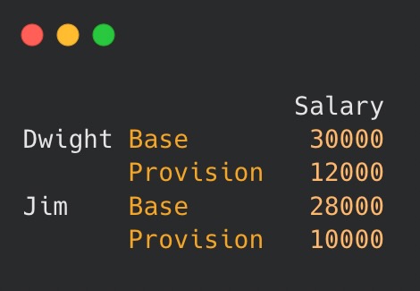
Retrieving data for a particular employee is also straightforward. Similarly to single-level indexes, we can use the following syntax: data.loc["Dwight"] or data.loc["Dwight", "Salary"] to locate the lower level of the index. 

Undoubtedly, MultiIndexing provides a flexible way to handle complex data structures as well as perform advanced data operations. However, one must remember that working with this feature can be more complex than with a single-level index, requiring more effort to understand how to effectively manipulate provided data. Lastly, it is worth noting that MultiIndexes consume more memory, which can become a concern if memory usage is a limiting factor to our application.

Validate data with pandera

Last but not least, when it comes to data analysis dedicated tools like pandas, one crucial feature that is often missing is type annotations. It is widely recognized that comprehending a written code tends to become challenging when there is no data type representation available. Fortunately, the pandera package provides a solution by allowing declarations of data structures for columns within pandas DataFrames as well as incorporating validation methods. This package aims to integrate data validation into the data analysis workflow, all while maintaining a simple, straightforward syntax.

In order to use pandera, we must install the package: pip install pandera. Upon installation, let us take a look at the following code:

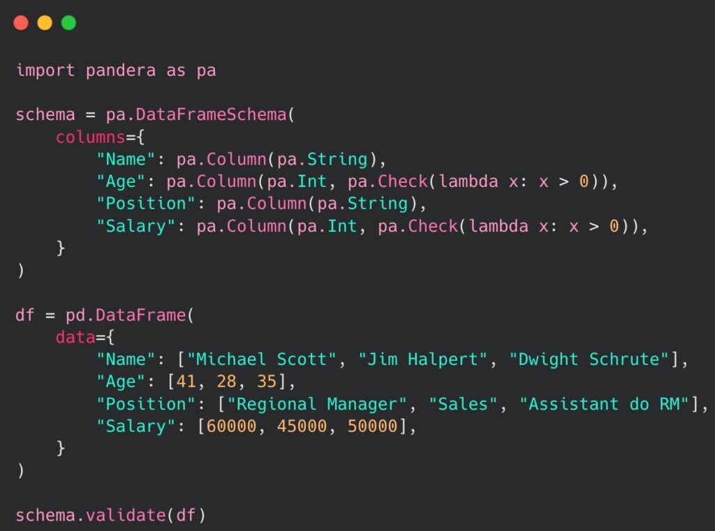
In the given example, we have utilized the DataFrameSchema object from pandera in order to define a desired structure and constraints for the data within the DataFrame. We have explicitly assigned the appropriate data types to each column and applied additional validation methods specifically for the integer fields in the declared DataFrame. The execution of the validate() method concludes the code and verifies the validity of the provided data. This is where any errors would be raised, whenever the DataFrame content fails to meet the validation criteria defined in the provided schema. If we provide a value to the Name column that would not be a string, an appropriate SchemaError would be raised. A validation error would also be raised whenever any value in the Age column would be less or equal to 0.

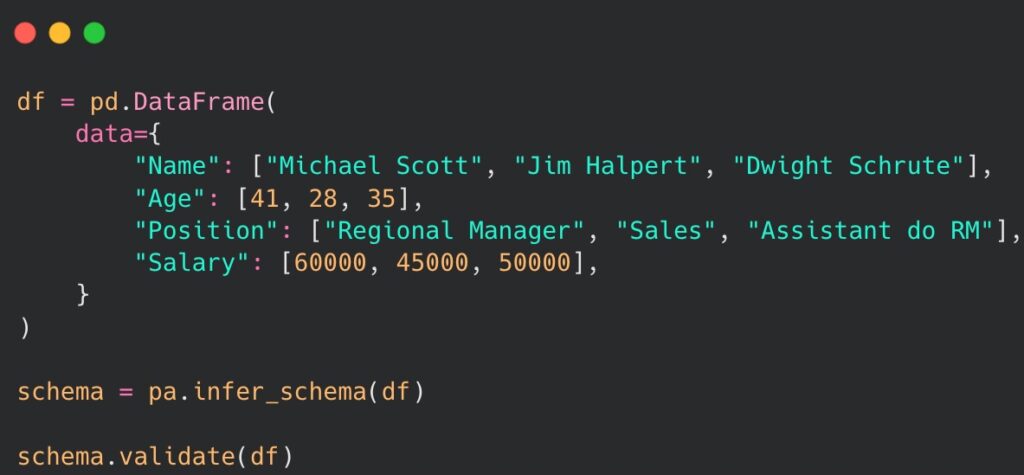
When custom validation of the data is not our priority, there is no need to explicitly define the schema. Instead, we can use a built-in method of pandera called infer_schema(), which attempts to guess the structure and the type representation of the given DataFrame. Unfortunately, we lose the custom validation capabilities of the explicitly declared schema. The following code presents an example:

Lastly, there is an option to perform it using a dedicated model to explicitly declare a schema, instead of the previously mentioned complex DataFrameSchema class. The solution is built on top of another widely used Python package for data validation – pydantic. The example of implementation is as follows:

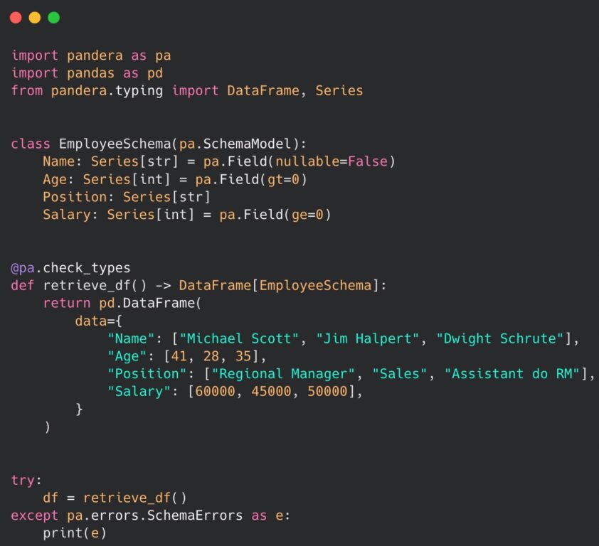
As observed, we have declared a class named EmployeeSchema with the initialization of data types as instance variables, representing the DataFrame structure. This approach is a much shorter and more readable representation of the schema. With the integration of pydantic, all the validation methods and key elements of that popular library are accessible and can be used conveniently in this context. We have also introduced a new function called retrieve_df() which incorporates the @pa_check_types decorator from the pandera package. This function allows us to specify the expected structure of the returned DataFrame by providing a declared schema model. By adopting this approach we can easily identify and handle any potential SchemaErrors that may be raised. Without a doubt, the provided examples serve as concrete evidence that implementation of pandera in our code can greatly simplify the process of validating the structure and data types of any DataFrame.

Summary

An undeniable strength of discovering the full potential of Python’s packages is knowing how to harness their capabilities by implementing at least some of their secrets and hidden gems in our code. I strongly believe that pandas, one of the most renowned tools in the Python ecosystem, will keep on surprising us while we continually reveal all of its mysteries. In the meantime, I trust that the insights shared in this article prove invaluable in our day-to-day developer’s work and make the life of a programmer at least slightly easier.